By Clare Leaver, Owen Ozier, Pieter Serneels, and Andrew Zeitlin

This post is also posted on the Development Impact blog.

The holidays are upon us. You might like to show off a bit by preparing something special for the ones you love. Why not make a pre-analysis plan this holiday season? You’re thinking, I do that every year, but we want to tell you about a new twist: using a dash of endline data!

Make a *what* this season?

Only slightly-less-well-known than the menorah, yule-log, and festivus pole, the pre-analysis plan is fast becoming a tradition. The merits and costs associated with such plans have been much-discussed, for example by Olken (2015) and Coffman and Niederle (2015). A well-agreed-upon merit of these plans is to keep various research misdeeds (of a p-hacking flavor) in check. (In line with your obvious goal for the holidays, not being naughty.) So, if you are feeling up to the task, how do you do it? A pre-analysis plan has many ingredients. Christensen and Miguel’s 2018 JEL article provides detailed guidance, but in this blog post we focus on a decision of under-appreciated importance: how to test hypotheses. Better still, we provide a recipe (and, as with any good cookbook, a couple of nice pictures to enjoy in case you don’t get a chance to try this yourself.)

What about what to test?

Decisions about what outcome to examine, and what hypotheses to test for that outcome, are of course important, but not the focus of this blog. These ‘what’ questions are typically guided by theory, policy relevance, and available data. They include an economic statement of the hypothesis, a choice of outcome variable and treatment, and a statement of the relevant null against which to test.

Didn’t we already know how to test?

No, you see. In economics, much of the thinking about the ‘how’ question has focused on choices of covariates and subgroups (see for instance Belloni, Chernozhukov, and Hansen, as well as the previously blogged Fafchamps/Labonne and Anderson/Magruder papers).  But that is not all there is to choose. Choices of test statistic are equally important for power, as Athey and Imbens (2017) recently discussed. Guidance is less well-established for researchers wishing to choose test statistics. This is where we come in.

Don’t you usually study development economics?

Yes, and that’s what led us here. In a recent experiment that tests the recruitment, effort, and retention consequences of pay-for-performance schemes in Rwandan education, we tried a relatively new approach: using blinded endline data to make these decisions. (For an earlier implementation of a similar idea in political science, see Humphreys, de la Sierra, and Windt.) The study allows us to test for pure compositional effects of (advertised) pay-for-performance contracts on the applicant pool, as well as effects on the characteristics and value added of placed teachers; because we apply a second randomization, it also allows us to compare the effort-margin response of these teachers to their realized contracts. We wrote down a simple theoretical model to help us understand these hypotheses, registered the trial, and then turned to blinded endline data to decide how to implement tests of these hypotheses.

Oh, do tell!

Well, the details of our experiment are not our focus here, so we’ll mention just enough to put our analytical approach in context — full details are available in our registered pre-analysis plan. The experiment is a two-tiered randomization. At the advertisement stage, we randomized job openings for civil service teaching positions to either receive pay-for-performance (“P4P”) or fixed-wage contracts. This was randomized at the (district) labor-market level. Then, after these teachers were placed in schools, we re-randomized contracts at the school level for both new recruits and incumbent teachers (buying out recruits’ expectations with a universal recruitment bonus; this second re-randomization is inspired in some ways by the design in Karlan and Zinman’s “Observing Unobservables” paper). This design allows us to compare value added among teachers recruited under different contracts, but who teach in the same contract — disentangling the compositional and effort-margin consequences of performance contracts.

Okay, fine. What part of that will help with this holiday project?

Our blinded pre-analytical work uncovered two decision margins that could deliver substantial increases in power: changing test statistics used and putting structure on a model for error terms. Because the value of these decisions depends on things that are hard to know ex ante — even using baseline data — they create a case for blinded analysis of endline outcomes. We argue that there are circumstances in which this can be done without risk of p-hacking, and in which the power gains from these decision margins are substantial.

THE RECIPE (be sure to have your apron on; this is where it gets serious)

 How can blinded data be used to assess power against specific alternative hypotheses? Consider, for example, a hypothesized additive treatment effect that is the same for all units in the sample. While the details of our experiment meant that we followed slightly different recipe variants for each of our outcomes (always have some caveats!), here is a general recipe:

1. HOW MANY PEOPLE ARE YOU PLANNING FOR?

(Ideally): If using data from only one arm of the study, such as the comparison arm, bootstrap a sample out of the available data, in order to work with a sample of the same size as the eventual analysis, and nest steps 2-3 below within repeated bootstraps. Otherwise, begin with the pooled data from all study arms, blinded.

2. PREHEAT OVEN TO DESIRED NUMBER OF SIMULATIONS, THEN BAKE

For each of R simulations, r = 1, … R :

a. Draw a feasible vector of treatment assignments, T_r.

b. Apply the hypothesized treatment effect to the data to obtain outcomes Y(T_r). This delivers a simulation of the data that a researcher would have in hand, if the hypothesized model were correct.

c. Calculate the proposed test statistic(s) for this simulation.

d. INGREDIENT SUBSTITUTIONS ARE POSSIBLE:

Make the accept-reject decision for this simulation:

i. If you are using an analytical distribution for testing (Z, Student’s t, Chi square, etc.), use that as the basis of your accept-reject decision.

ii. If using randomization inference (as we are), the accept-reject decision for this simulation should be based on comparing the test statistic (from Step 2c) to the distribution of that same test statistic that a researcher conducting RI would have computed, if they held the presently simulated data in hand. So, for each of P permutations, draw yet another alternative treatment assignment but keep the data, Y(T_r), generated by treatment draw r. Calculate the test statistic(s) of interest for that permutation p. Use the distribution that results from the P permutations to make your accept-reject decision.

3. LET COOL BEFORE SERVING

Power against the specific alternative hypothesis is approximated by the share of rejections across the R draws of the treatment assignment used to generate simulated data.

4. Add additional caveats; season to taste.

Caveats?  Do you have any favorites?

Sure. For example, notice that if you begin with all study arms of pooled, blinded data, then these data are a good simulation of the distribution of outcomes under control *only* if the sharp null of no treatment effect for any unit is actually true in the experiment.  Otherwise, the fact that they embed a mixture of potential outcomes from different treatments will make this an inaccurate representation–more so the more the treatment changes the distribution of outcomes; bootstrapping up from just the comparison arm might have been better.  On the bright side, under the sharp null, this would produce precisely the randomization inference distribution that will eventually be used.  Thanks to Macartan Humphreys for discussion of this point, in relation to this recent blog by Cyrus Samii.

Sounds delicious!

See? Easier than you thought. What kinds of things can be learned from such an exercise? (What is the nutritional value?) We illustrate this with two examples, with full details of each provided in our Pre-Analysis Plan.

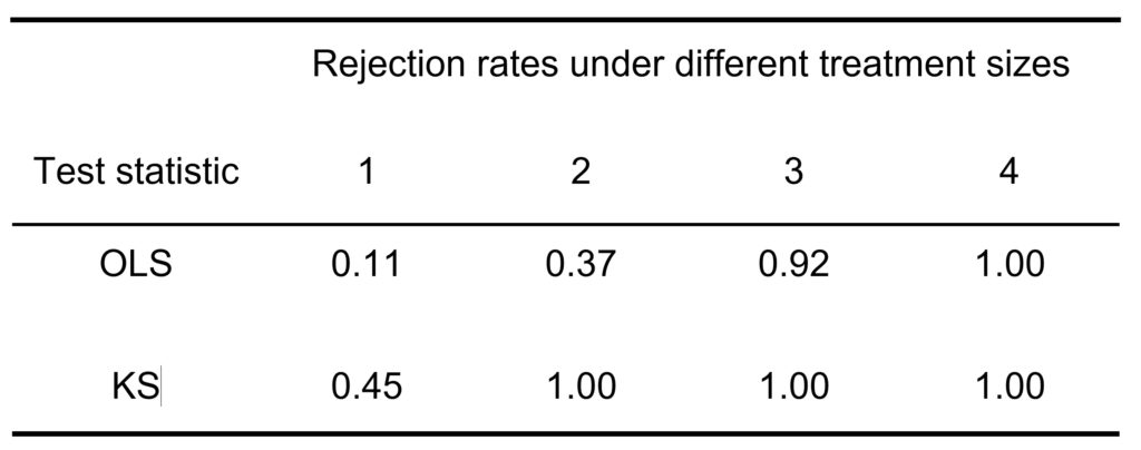
RESULT 1:  Kolmogorov-Smirnov (KS) tests can be better powered than OLS t-tests by a factor of four, even under additive treatment effects.

A first application for us is the effects of the advertised (randomized) contract terms — P4P or fixed wage — on applicant quality, measured by teacher training college exam scores.  Because hiring is (thankfully) not at random from the distribution of applicants, we knew from the outset that mean application quality was not the most policy-relevant statistic, so we planned to use a KS test to test for differences in distributions (which we might map through alternative hiring rules to potential qualities of hires). But power to detect differences in means remained important to us. This left us with a question: if the truth were an additive treatment effect (subject to exam scores being bounded between zero and 100 percent), would an OLS t-statistic outperform a KS test on these outcomes?

The answer, presented in Table 1 below, surprised us. Simulated rejection rates were much higher when using a KS test, even when the hypothesized treatment effect was additive. Because there are no comparable ‘baseline’ applications, we could not have learned this without access to endline data.

Will my plan turn out this way?

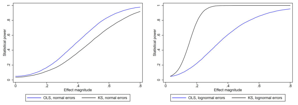
Maybe; the relative power of KS to reject additive treatment effects is not unique to our setting. As an example, it is easily shown that KS rejects an additive treatment effect at a rate higher than OLS when control outcomes are log normal.

For more general cases, the lesson we take away here is that the consequences of the distribution of outcome data for the relative power of alternative test statistics may be large and hard to anticipate.

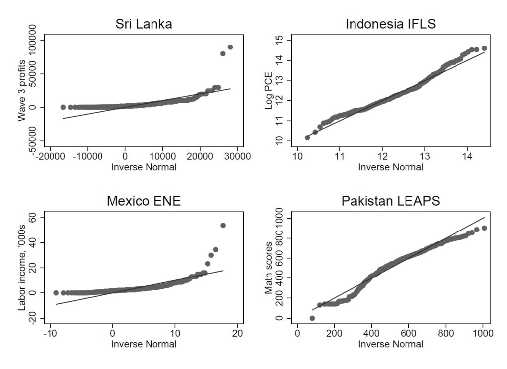
We looked at data from Bruhn and McKenzie (2009), and saw that departures from normality are common across typical outcomes in development:

See also Rachael Meager’s approach to non-normally distributed microfinance profits. So what kind of outcome distribution are you cooking with? That’s for you to find out.

Yes, but my outcomes are normally distributed. What is this recipe doing for me?

Ah yes. Traditionalists like to focus on cooking classic dishes. We understand. Read on!

RESULT 2:  Linear mixed-effects models sometimes outperform alternatives by expressly modeling unobserved variation.

Remember how machine learning is a way of getting a better fit using observables?  Imposing structure on error terms is a way of getting a better fit on the *unobserved* sources of variation.  That structure can take many forms: it can relate to the correlations between units, the distribution of residuals (normal? pareto?), or both.  Imbens and Rubin (2015, p. 68) observe that test statistics derived from structural estimates — for example, expressly modeling the error term — can improve power to the extent that they represent a “good descriptive approximation” to the data generating process. Blinded endline data allowed us to learn about the quality of such approximations, with substantial consequences.

In our setting, when we turned to look at effects on student outcomes, we intended to use a linear model (y = x beta + epsilon, but a little longer).  But there were still a number of potential correlations to consider: some students are observed at more than one point in time; each student has multiple teachers, and schools may have both incumbents and teachers recruited under a variety of contract expectations. Linear mixed-effects (LME) models provide an avenue for implementing this.

Our LME model, which assumes normally distributed error terms that include a common shock at the pupil level, delivers an estimator of the effect of interest that has a standard deviation as much as 30 percent smaller than the equivalent OLS estimator.  Because normality is a reasonable approximation to these error terms, the structure of LME allows it to outperform traditional random-effects. The gains from LME are conceptually comparable to an increase of 70 percent in sample size (because the square root of 1.70 is about 1.30 – and we’re the sort of people who get excited about square roots)!

SOME PARTING THOUGHTS (before you go out shopping for ingredients)

Is there something in this recipe my third cousin might find disagreeable?

Of course! This approach is not without risks. Some of these apply in other circumstances, too. For example, even when researchers submit pre-analysis plans based on baseline data only, they commonly have at least a qualitative sense of some issues, like compliance, that may inform choices. But some concerns are specific to the use of endline data. When the distribution of an outcome is known in one arm, even blinded, pooled data can allow researchers to update their beliefs about the treatment effect on a particular outcome; David McKenzie and Macartan Humphreys discussed this in a blog post and comments in 2016 here. There are likely to be solutions to these issues, such as registering outcomes prior to endline, using the blinded dataset only to inform the how question, or using data from a single treatment arm rather than pooled data.

What have we learned?

Endline data are often far from normal and correlation structures across units are hard to know ex ante. A blinded endline approach can be a useful substitute for tools like DeclareDesign in cases where baseline data, or a realistic basis for simulating the endline data-generating process, are not available.

There is broad consensus that well-powered studies are important, not least because they make null results more informative. Consequently, researchers invest a lot in statistical power. Our recent experience suggests that blinded analyses — whether based on pooled or partial endline data — can be a useful tool to make informed choices of models and test statistics that improve power.

Don your ugly sweater. On your marks, get set, bake!

(and over to someone else for dessert)

Thanks to Katherine Casey, Dean Eckles, Macartan Humphreys, Pam Jakiela, Julien Labonne, David McKenzie, Berk Özler, and Cyrus Samii, for helpful conversations and comments as we developed this blog post.